Bayesian Neural Networks

Giving a neural network the ability to undermine it’s own confidence

Neural networks are complicated objects already. I’ve been wanting to delve into creating a Bayesian neural network for some time to extend my range in Bayesian methods. A Bayesian neural network complicates things further by using distributions with their own number of shape parameters for each neural network parameter, increasing the number of total parameters and training cost.

I used the MNIST dataset to for this project because its a solid choice for experiments and is easily downloadable. The MNIST dataset is a collection of 28x28 mono-color images of handwritten digits 0 - 9. There are 60,000 training images and 10,000 test images. Some example images are illustrated below. The neural network I will construct here is a dense neural network. This means the shape of the MNIST images is not preserved. Instead, the images are flattened to a one-dimensional vector that we feed into the neural network for training.

I am building this neural network using Tensorflow, and within that, Keras but the standard Tensorflow package does not include methods and functions necessary to integrate Bayesian statistics into a neural network. The package I needed was Tensorflow-Probability, which is easily installable with pip in python3.

Most of the layers in this neural network are all found in the Tensorflow library. This neural network used a Flatten layer to quickly turn the 28x28 pixel MNIST digit images into length 784 vectors. There was also a Dropout layer in between each hidden layer that was added. The probability for all dropout layers was 0.25.

Tensorflow-Probability provides the relevant layers we need to perform Bayesian statistics, namely: - DenseReparameterization - OneHotCategorical

Here is the main difference between your standard neural network (i.e. an input layer, some hidden layers, an output layer) and a Bayesian neural network. Rather than having a matrix of single value weights W_{1} … W_{n} for your trained neural network, those matrices are now sets of distribution parameters for each weight term. If those weights can all be represented by a normal distribution with a mean and a standard deviation, then each weight term now has two values. Additionally using the bias distribution in the DenseReparameterization layer will add two more values (again, depending on your distribution of choice) per bias term. The image below illustrates how the weights and biases in the nodes of a simple neural network compare with a Bayesian neural network.

Now in using the DenseReparameterization layer in your neural network you need to specify a prior distribution for your weight distributions. In this case I set the prior for both the weights and biases to a standard normal distribution with some mean and some standard deviation to keep things simple.

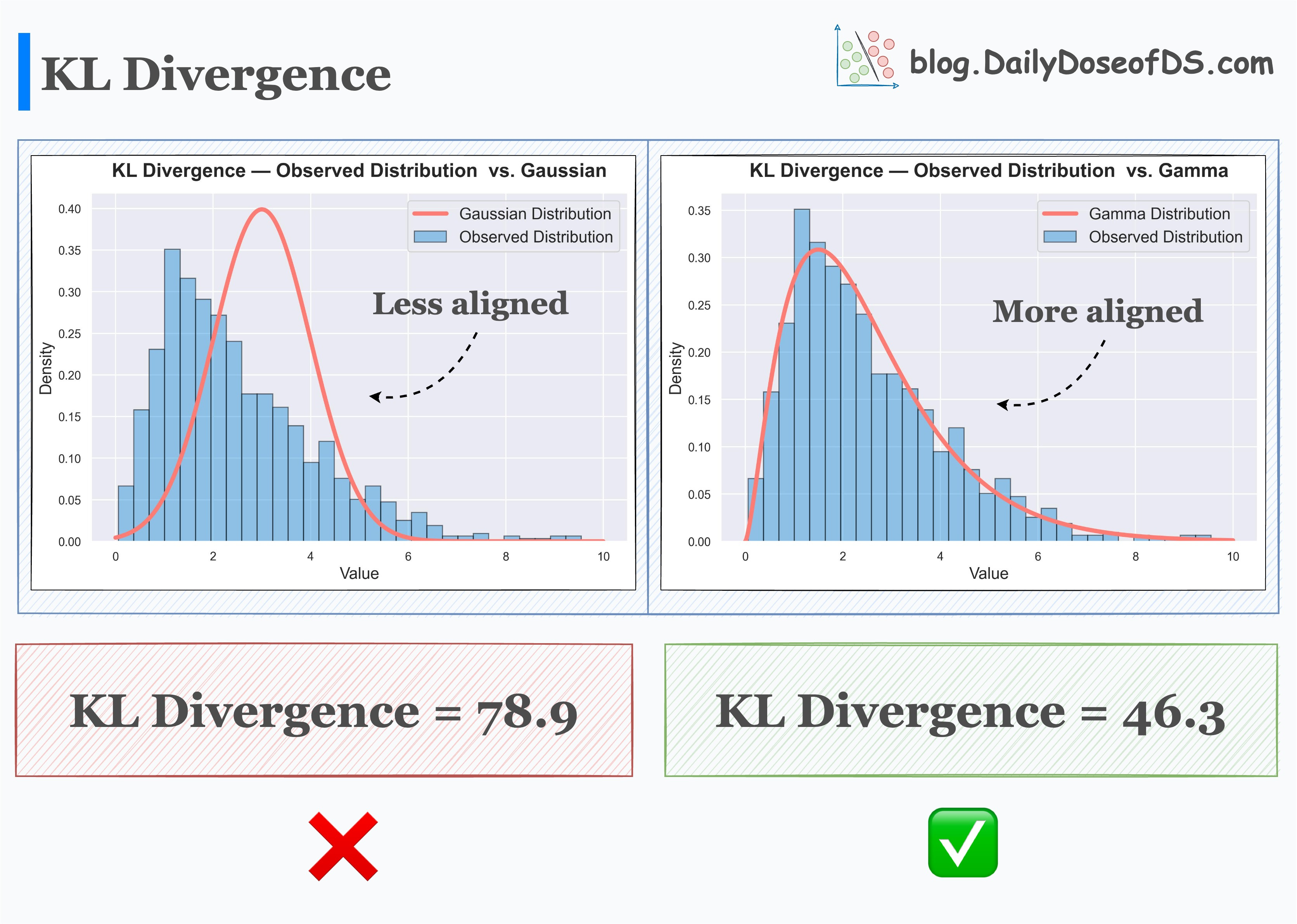
You also need to specify a function to calculate the divergence for both weights and biases. All this means is for each pass, you’re comparing the joint distribution of your priors with what your neural network is currently generating. In keeping things simple I opt to use the Kullback-Liebler divergence for this job. I’ve linked a handy image from Daily Dose of Data Science below illustrating how the KL divergence quantifies how one distribution compares to another. The smaller the KL divergence value the better your two distributions match each other.

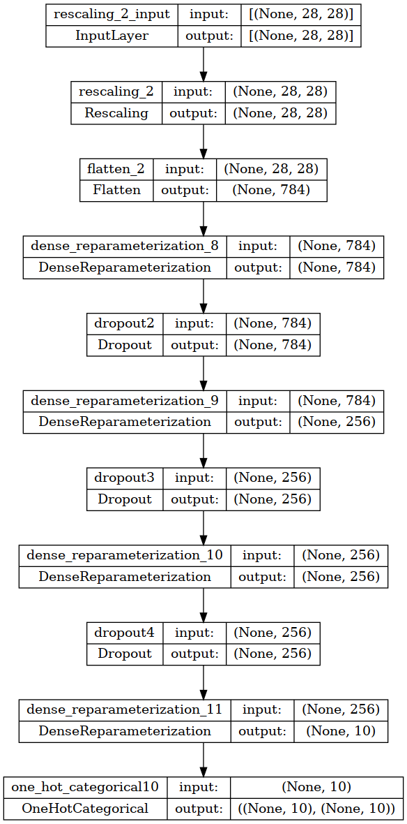
The model architecture is pretty straight forward; two pre-processing layers, 4 hidden layers with 25% in between each layer. Finally an output layer from which we get our predictions from. We have one rescaling layer to change pixel values from 0-255 down to 0-1 for better numerical stability. Following that is a flattening layer that turns each 28x28 MNIST image into a 784 entry 1-D vector. The actual model follows here with 4 Dense Reparameterization layers with 784-256-256-10 units in that order. Finally there is the output layer which outputs the one-hot categorical probability.

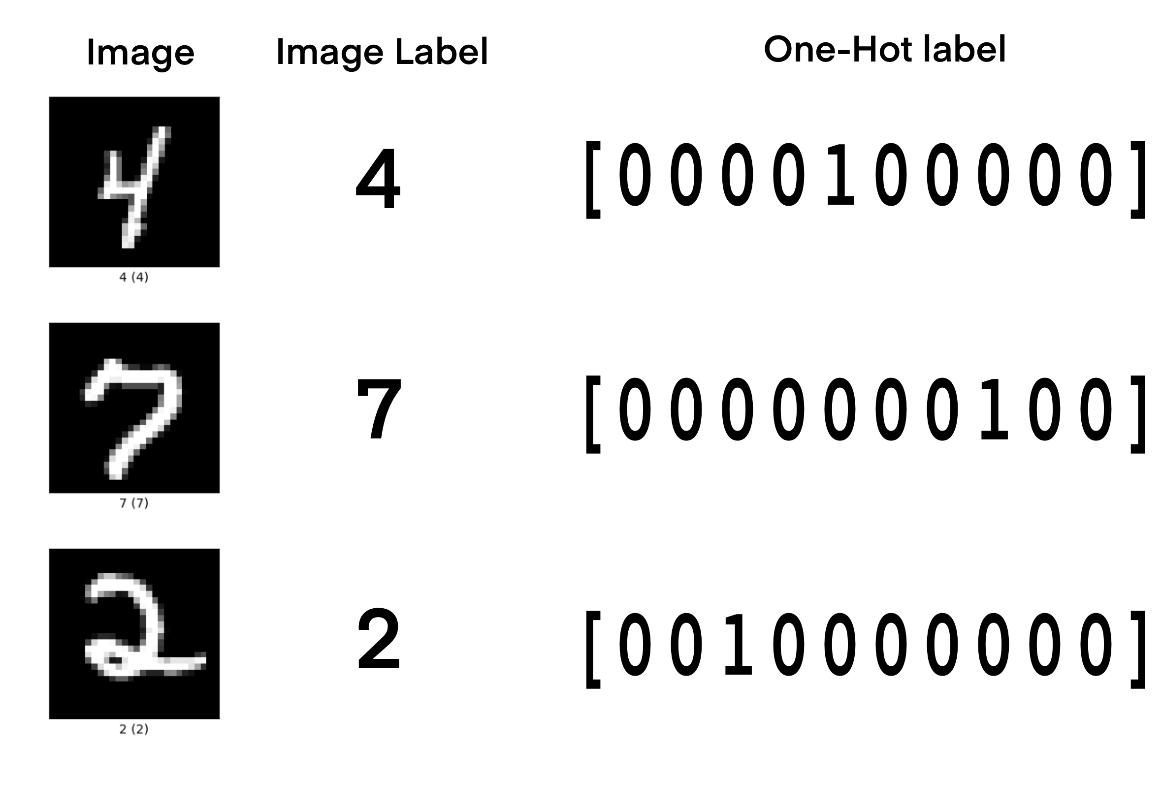
One-hot encoding here is another choice in data pre-processing which increases numerical stability. Our MNIST digit image labels range from 0 - 9, but this can lead to instabilities in training. We can convert the MNIST digit image labels to a vector of size 10 where the ith number corresponding to the image label is ‘1’. This preserves the labels for training and gives the model more information about the label structure. An image illustrating how one-hot encoding works is below.

Below is a small summary image of the neural network architecture using the Keras ‘plot_model’ utility (click on the image if you’d like to see it fullsize). This model has a total of 1,769,524 parameters. The same model architecture using the Keras ‘Dense’ layers without any Bayesian capability has a total of 884,872 [parameters. Dividing 884,872 by 1,769,524 is about 0.5000(6) which is a neat validation of how Bayesian parameters scale compared to regular parameters in a neural network, at least when using Normal distributions.

I compiled this model to use the negative log-likelihood as the loss function instead of ‘CategoricalCrossentropy’ which would be used in the non-Bayesian model. The optimizer is the Adam optimizer with a low learning rate of 1e-4 (or 0.0001).

The model training is performed with a batchsize of 512 images per training epoch for both the training and validation sets for a maximum of 100 epochs and with an ‘earlystop’ callback to stop model fitting when there is no longer any improvement in the validation accuracy.

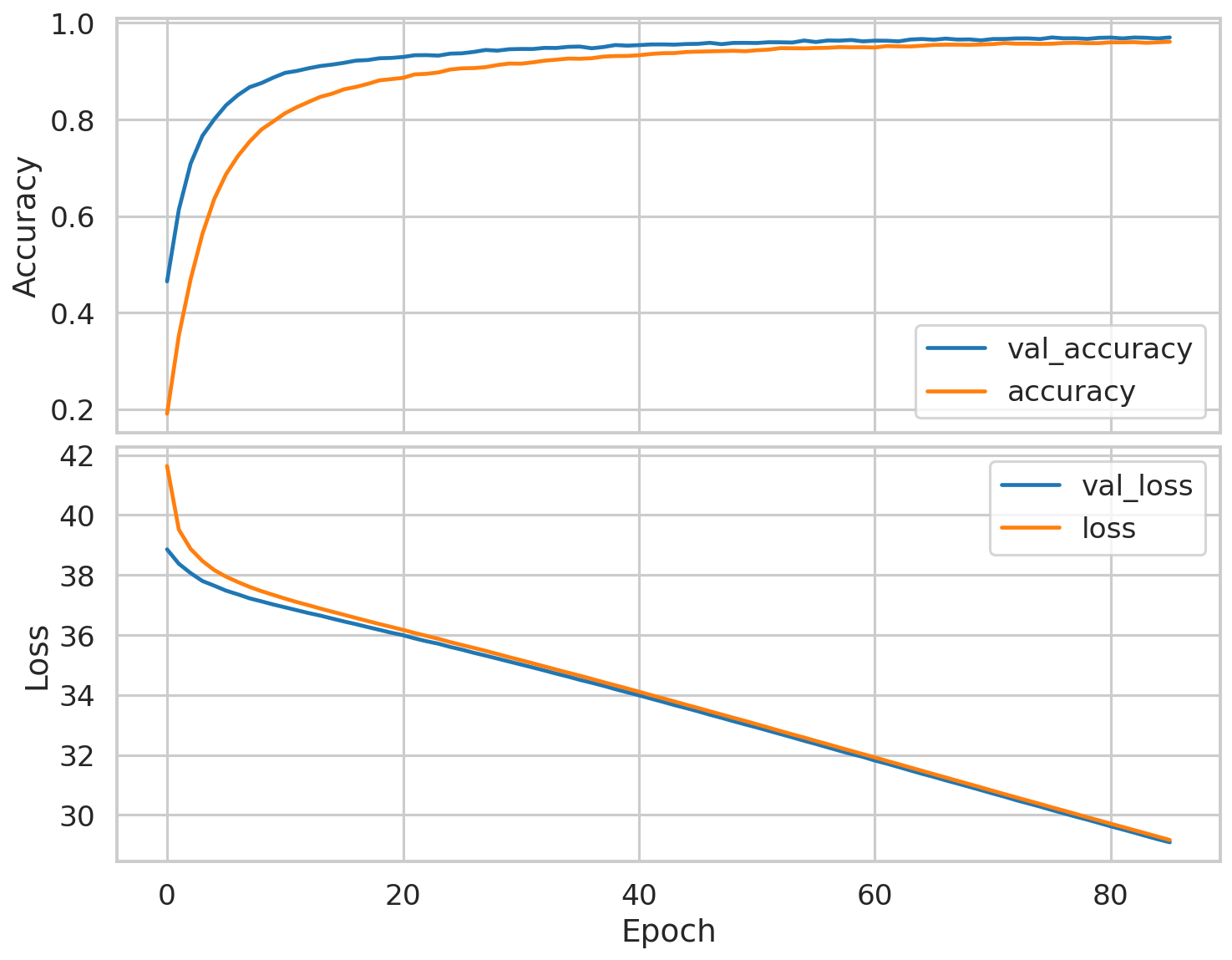
The model trained for a total of 86 epochs after at which point it achieved an accuracy of 96.1% and a validation accuracy of 97.1% which is a good indication that model doesn’t over/under fit too much. A vertical two-panel plot of the accuracy and loss evolution over training for the training and validation sets of this model is below.

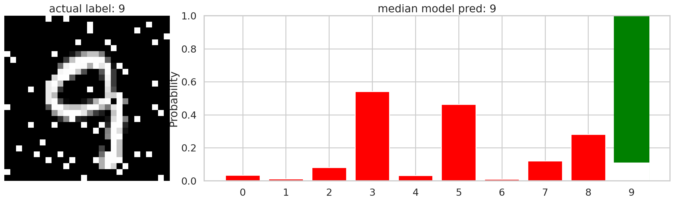
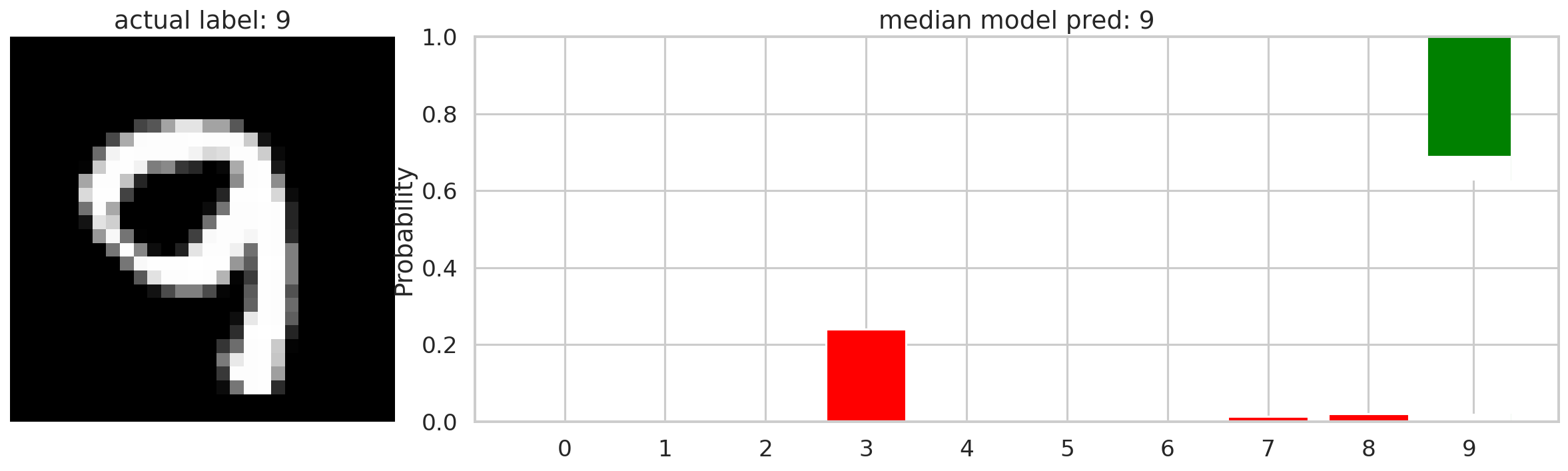
Now we can explore what Bayesian neural networks are very good at: giving you ranges of probabilities for classifications. The plot below illustrates how this neural network classifies an MNIST image of the number 9. The bar graph is the individual probabilities of each classification from the neural network’s predictions. The top of each bar is the 97.5 percentile of probabilities and the bottom of each bar is the 2.5 percentile of probabilities. The distributions of probabilities represent how the model identifies this vector over the distributions of it’s weights. If you wanted more information you could plot this with violin or box and whisker plots to display more structural information of each probability distribution.

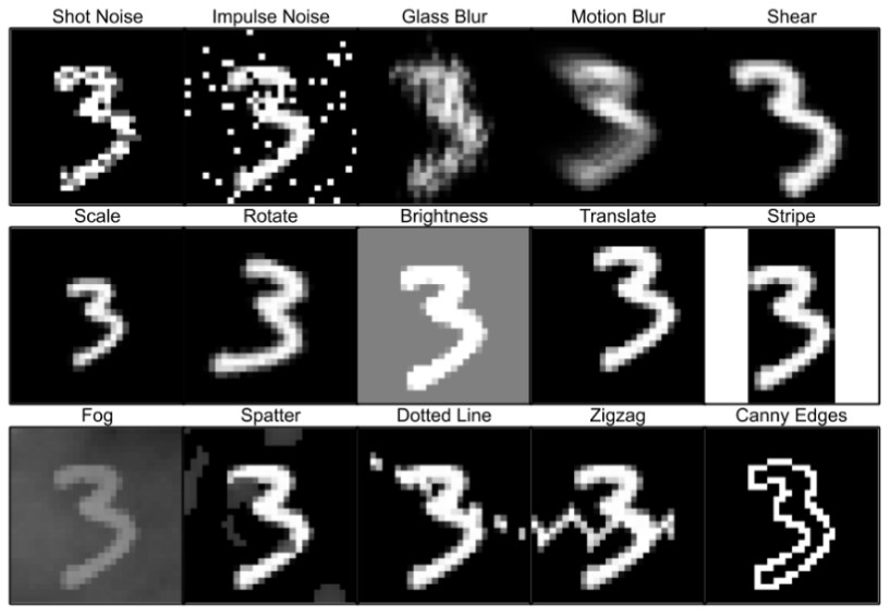
One last thing I’d like to demonstrate in this post is how this type of neural network can classify similar images that it has never been trained on before. In this case I use the MNIST-C dataset, which is a ‘corrupted’ version of the MNIST digit images. In this dataset the standard MNIST images have added visual artifacts to similar different image issues such as smearing, shot-noise, scaling differences, etc. An example image of corrupted MNIST images is added below.

If we feed the neural network a similar but corrupted image of the number 9, we get something like the image below. The neural network here still classifies correctly as the number 9, but the probability distribution is much wider, indicated a higher level of uncertainty in it’s prediction. There are now additional predictions to other numbers, each with their own probability distribution, further demonstrating that the neural network is not completely certain the image is the number 9. Having this type of additional insight into the neural network’s performance can further enhance it’s capability.