Autoencoder Neural Network

A needle in a haystack costing billions of dollars

This is part of a data science challenge project I have undertaken as part of the Correlation-One Data Skills for All bootcamp that I started back in October. I enjoy how well structured the bootcamp is to simulate industry specific projects to bolster professional skills in data science.

Credit card fraud, despite constituting less than 1 percent of all transactions, cost consumers more than 8.8 billion dollars in 2022 according to the Federal Trade Commission. At least 26 percent of adults in the United States were affected by fraudulent transactions, with estimated losses over 180 million dollars a year.

I took part in the data scientist section of this data challenge, which was to build a machine learning model that could effectively discriminate between fraudulent transactions and legitimate transactions. Before I could do that, I needed to analyze the 3 data sets that I was provided for insights. Then I had to clean the datasets for quality assurance, and perform data engineering to construct features. These features would then be scaled and fed to models that can best separate legitimate transactions from fraudulent transactions.

The three datasets are credit card fraud datasets from Kaggle that have been filtered to only contain transactions from 2016 - 2019 for 2000 customers.

• Credit Card Customer Data (2000 rows x 18 columns)
• Credit Card per Customer Data (6146 rows x 13 columns)
• Credit Card Transaction Data (6,877,837 rows x 15 columns)

The sizes of the transaction data proved to be a little troublesome to operate with in a jupyter notebook as it regularly crashed my python kernel until I remembered to run the notebook with plenty of extra memory which avoided the issue entirely. I found that keeping track of memory usage and converting data types to reduce memory usage sped up the subsequent analyses consierably.

The credit card customer dataset contains some demographic information such as location, gender, birth year, and some financial information like yearly-income, total debt, and FICO scores.

The credit card per customer dataset has multiple rows for each customer listing out each individual credit card in their name. Also included are financial details such as credit limit and credit card PINs and meta data such as the number of times a card has been reissued (due to loss, damage, theft, etc.).

The transactions dataset is the largest, containing all of the individual transaction assigned to each customer’s identity. It contains a Fraud column that labels each transaction as fraudulent or legitimate. There are only about ~8400 fraudulent transactions among the 6 million rows of legitimate transactions.

Data analysis consisted of exploring the columns of each dataset as well as joining the customer and credit card datasets to the “main” transaction dataset to better see what features can be engineered to best train a model. Some of the figures from that analysis are below.

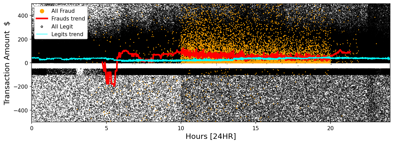
Figure 1 above shows the legitimate transaction amounts plotted by their 24 HR time of occurence as well as the occurence and amounts for all of the fraudulent transactions. The data itself doesn’t give us much insight, but the rolling median trend lines for each set show some structure. The legitimate transactions show a near a constant trend of amount spent across the entire 24 HR time range, whereas the rolling median amount for the fraudulent transactions shows more activity in the early morning hours and has more variation overall than the legitimate transactions. This quantitative information can be useful to a model to sus out differing characteristics between legitimate and fraudulent transactions.

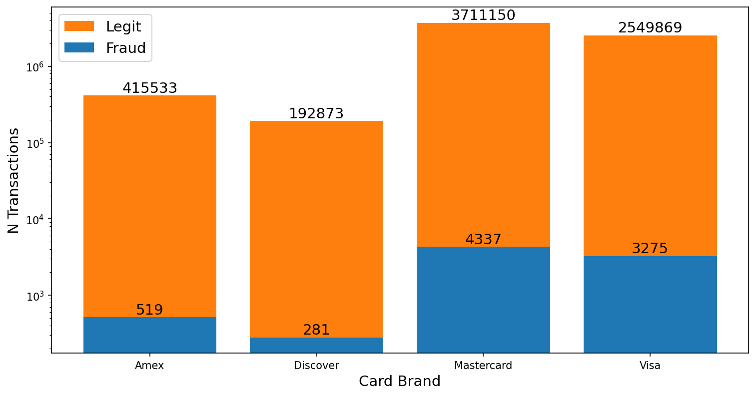
Figure 2 shows a bar plot of the total number of transactions grouped first by the credit card company that issued the card used in the transaction: Amex, Discover, Mastercard, and Visa, and secondly splits the total number of transactions into a legit number and fraudulent number. Fraudulent transactions appear to occur more frequently with Mastercard and Visa, moreso than the relative scale of the legitimate transactions between all four card companies. Categorical data like this is useful to a machine learning model to better identify fraudulent transactions.

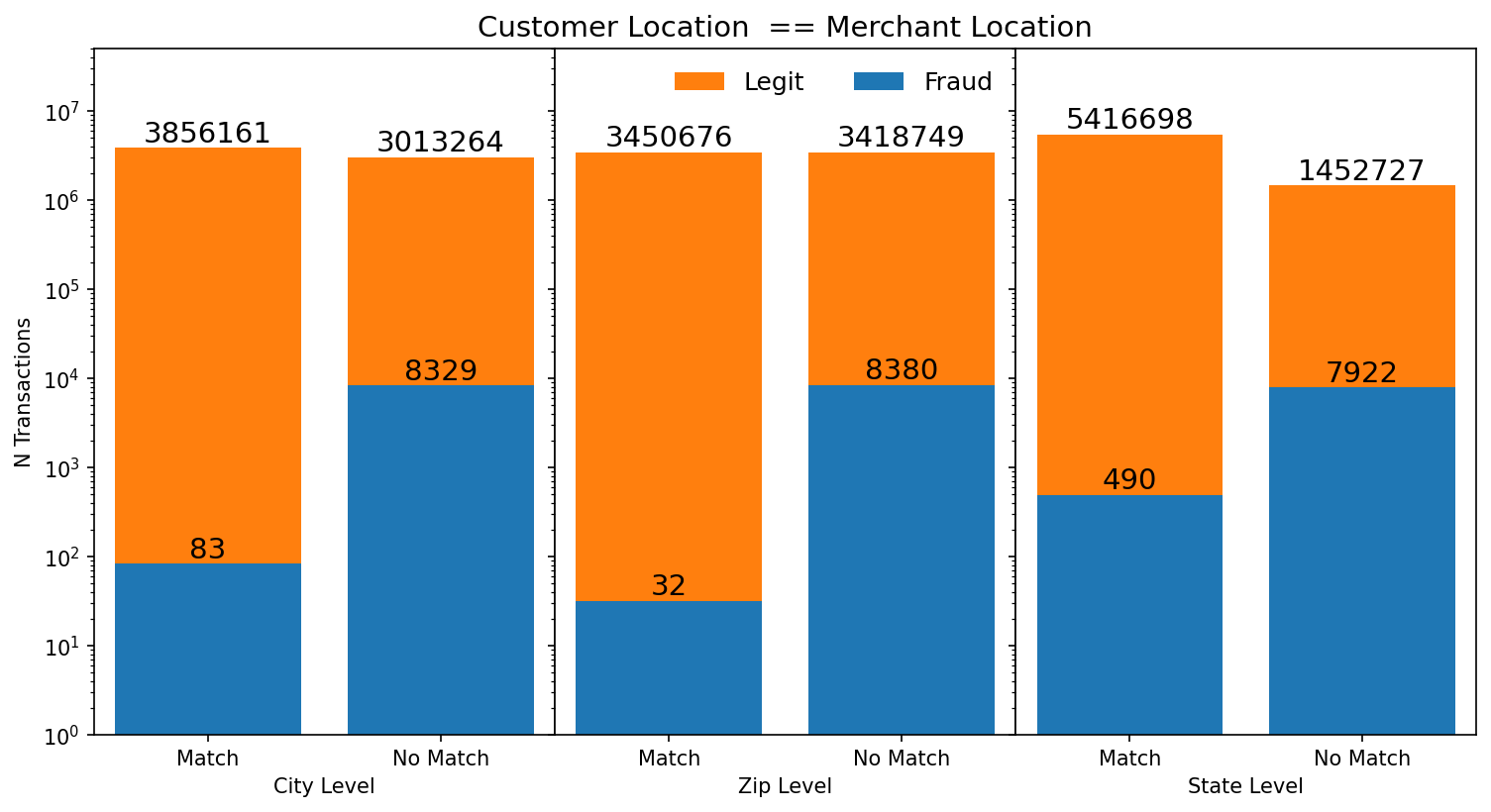
Figure 3 is a bar plot showing the total amount of transactions at the city, zip, and state level and whether the customer and merchant location at that level match. Furthermore the bars are split into legitimate and fraudulent transactions. Fraudulent transactions appear to take place more frequently outside of the customer’s location at all 3 levels, with the biggest difference at the city, and zip-code level. The state level doesn’t display as much difference in the number of fraudulent transactions when the state location doesn’t match as opposed to when it does. These features were engineered by me from the categorical columns in the dataset and can serve as custom categorical features for a model to train on.

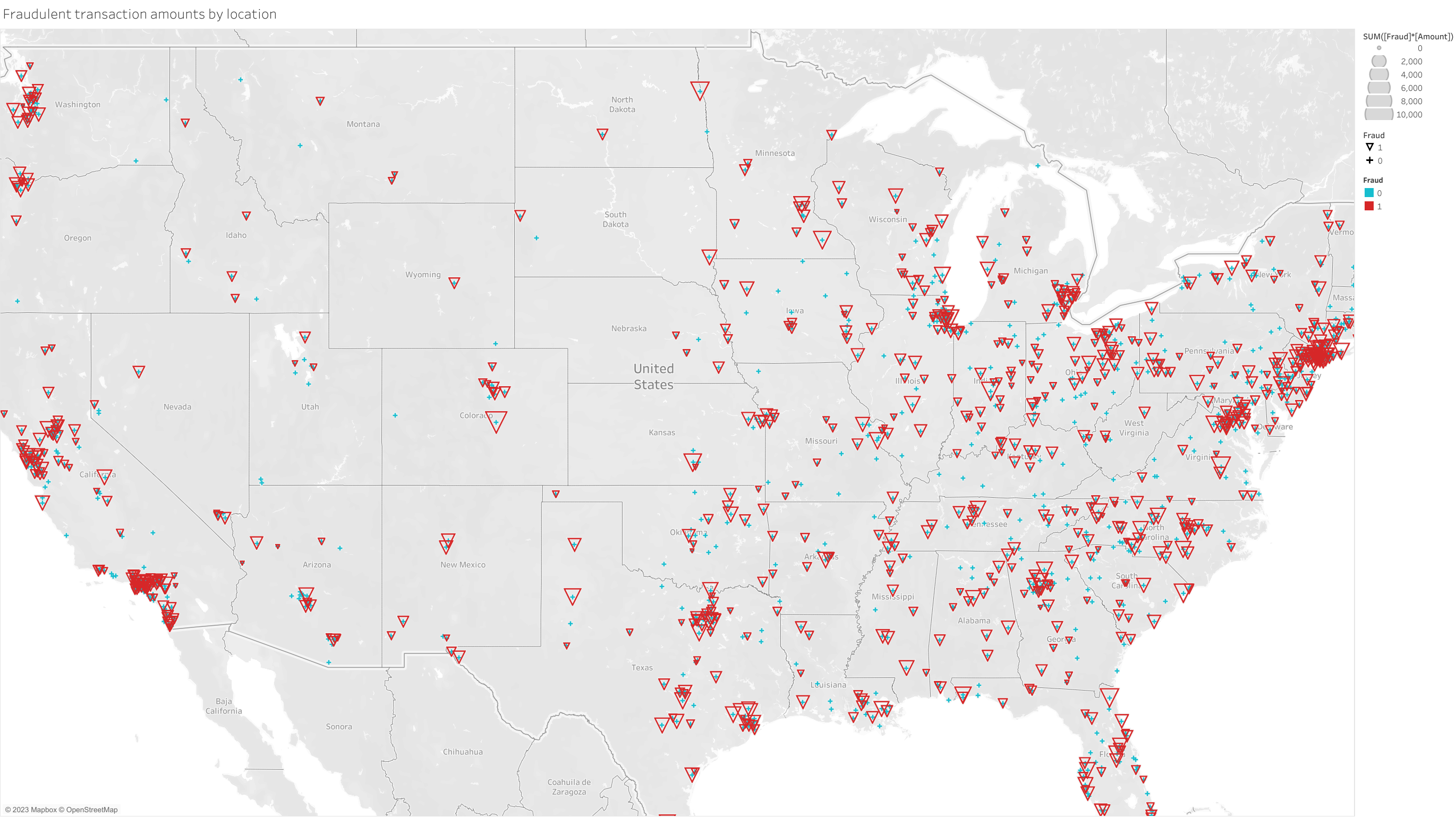
Figure 4 is a geographic map plot of the United States illustrating major areas of fraudulent transactions in red triangles, sized by the sum total amount of money involved in the fraudulent transactions. This figure shows that major metropolitan areas on both coast lines, as well in some inlying ares like Chicago, Illinois and Dallas, Texas. It would be too involved to train a machine learning model to consider geographic locations to try and separate out fraudulent transactions. However boolean features as to whether the customer and merchant locations match at different levels can provide the same amount of information without needing a geographic context in a model. This figure was exported from tableau and is available to interact with in a dashboard in my Data and Visualizations project page.

I engineered 56 features for each transaction, including quantitative features such as the ratio of each customer’s income to their total credit card debt, the total time between a transaction and that credit card’s last PIN reset, categorical features such as the card brand, customer-merchant location matching at different levels, and simple boolean features such as the error type (if any) present in a transaction.

The quantitative features were scaled to unit variance using SciKit-Learn’s quantile transformer, which is robust to outliers so as to avoid outlier filtering, as I wanted to keep as many outliers as possible that may be indicative of fraudulent transactions. With over 6 million transactions, I sub-sampled 3 million of the legitimate transactions, and all 8412 fraudulent transactions to be used for my model. This was split into training, validation, and test sets following a 50% : 25% : 25% ratio. The ratio of fraudulent transactions to legitimate transactions in each subset comes out to around 0.5% which I left unmodified for the validation and test sets. The training set had the fraudulent transactions upsampled to constitute 10% of the training set using the Imbalanced Learning python module, IMBLearn. Upsampling up to 10% better helped the model converge towards a better separation of legitimate and fraudulent transactions.

I decided to use (as my project title states) an autoencoder neural network architecture as my model of choice. I first attempted to build a straight-forward dense neural network but found the effort not worth the returns. I performed supervised training by giving the autoencoder the fraud labels provided with the data as well as the 56 training features.

Autoencoders work by stacking two neural networks together to minimize the reconstruction error between the input data and it’s copy in the output data. The encoder reduces the dimensionality of the input data to some smaller shape. The decoder takes this smaller dimensional data and reconstructs it to the same shape of the input data. The reconstruction error decreases as the model learns how best to deconstruct the input and reconstruct it later. The model will learn what features are important for the most accurate reconstruction.

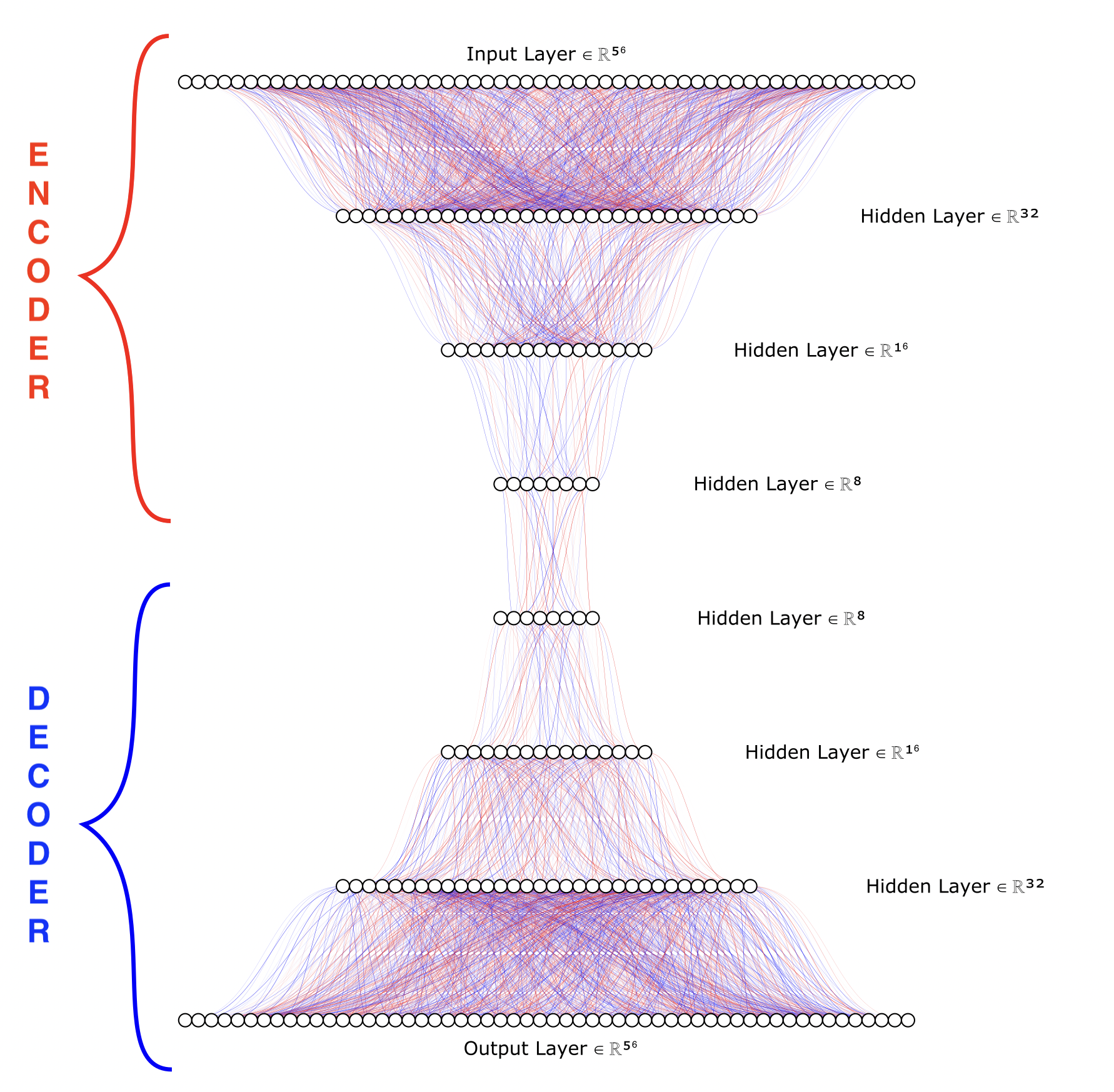
The final model architecture for the autoencoder I built was relatively simple. A four layer encoder where the data’s dimension is reduced from 56 to 32 to 16 and finally to 8. The decoder is the mirror image of the encoder but in reverse, going from 8 to 16 to 32 and back to the original size of 56. The final model architexture is plotted below in figure 5.

The loss metric used to drive the model’s learning was the mean absolute error, which I found performed best compared to the mean squared error, or the binary cross-entropy. I added L1 and L2 regularization terms to the encoder layers, and found the best values for L1, L2, and learning rate by running 100 trials of different values in a random search where each trial model trained for 10 epochs. The best model was trained for a maximum of 30 epochs but stopped training early at 27 epochs as the model was no longer learning further.

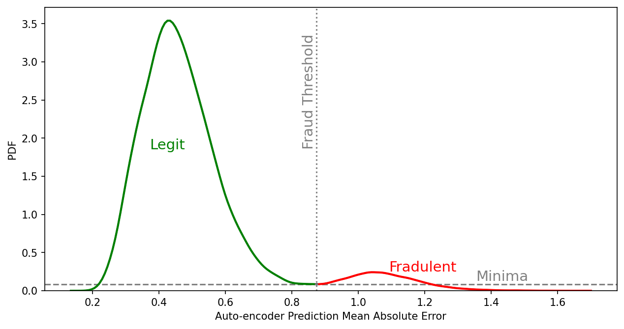
The test sets were fed into this trained model where each transaction has an associated mean absolute error in reconstruction between the encoder and decoder. A threshold in the distribution of the mean absolute error is needed to delineate the mean absolute error that describes legitimate transactions and that of fraudulent transactions. I found the best threshold by performing kernel density estimation on the values of predicted mean absolute errors and found the minima between the two peaks of the distribution. Figure 6 is a plot of that mean absolute error distribution for the test set with the threshold labeled.

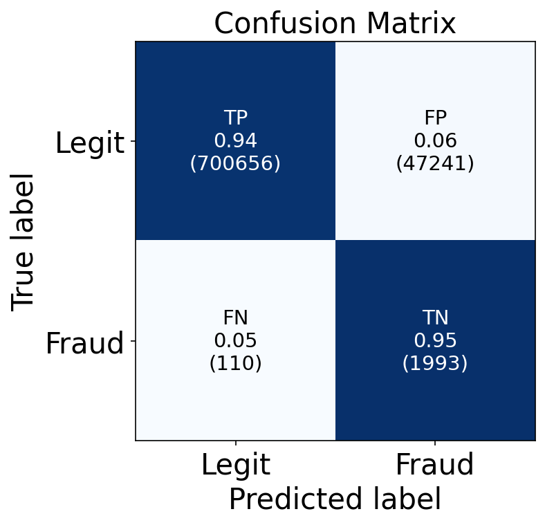
I convert these mean absolute error values to class labels by applying this threshold to the test set predictions. I quantify model performance by constructing a confusion matrix of the autoencoder’s predicted labels to the true labels in the test set below in Figure 7. Overall, the autoencoder performed well. The model achieved a 94% (700,656) true positive rate in identifying legitimate transactions and a 95% (1993) true negative rate in identifying fraudulent transactions. The nature of fraudulent transactions being rare but not impossible means that the percentages of false positives and false negatives have to be considered as more than percentages. Only 6% of legitimate transactions were classified as fraudulent, but that amounts to over 47,000 transactions. The 5% false negative fraudulent identifications amount to only 110 fraudulent transactions pass by without being detected. Ultimately the decision to further redesign the model to produce less false positives or less false negatives is up to me. Do I want to better identify legitimate transactions so as to conserve the resources in investigating possible fraud? Or do I want as many fraudulent transactions as possible no matter how many other legitimate transactions get flagged, possibly resulting in more resource usage and some annoyed customers?