
Bayesian Transfer-Learning with Feature Extraction
You can now interact with the featured Bayesian Neural Network at this Streamlit Web App
Introduction and Context
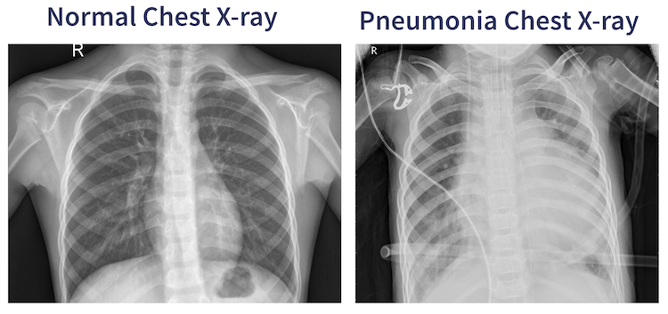
Pneumonia is an infection wherein one or both of the lungs are incapacitated by fluids in the air-sacs of the lung. Pneumonia accounts for about 2 million deaths yearly in children under the age of 5. Pneumonia is usually diagnosed by examination of chest X-rays wherein Pneumonia appears as cloudiness within the lungs.
Automated medical image diagnoses streamlines the usage of human medical resources. In this case a radiologist who visually inspects the X-rays to see if there is the presence of pneumonia. In the visual inspection case this radiologist would give equal attention to each image they receive, and issuing a diagnosis or lack thereof. It’s more important for the radiologist to give their attention to the possible pneumonia x-rays. An AI system that could pre-classify chest X-rays could expedite the diagnostic workflow of the radiologist and reduce times between examination, diagnosis, and more importantly, treatment.
The Data
The dataset I use in this project comes from the Large Dataset of Labeled Optical Coherence Tomography (OCT) and Chest X-Ray Images which looked at using transfer-learning in order to explore the feasibility of early detection of specific ailments that are typically diagnosed from visual examination of X-rays. I quote the two main sections of text that best describe the Pneumonia dataset, as well as the methods of labeling that were used in the shaded text boxes below.
The original authors of the Cell article this dataset originates from achieved an overall accuracy of 92.8% in correctly classifying the data set, with a sensitivity of 93.2% and a specificity of 90.1%. Sensitivity is essentially “What fraction of people with an illness were correctly identified as having an illness?” Specificity can be phrased as “*What fraction of non-ill people were correctly identified as not having any illnesses?” These last two metrics are what are typically cited in medical settings for the performance of a diagnostic test since it’s most relevant. Later on I will calculate these same parameters to see how my model setup performed and also include uncertainties on these estimates due to the Bayesian nature of the dense bottom layers I will be using.
Description: "We collected and labeled a total of 5,232 chest X-ray images from children, including 3,883 characterized as depicting pneumonia (2,538 bacterial and 1,345 viral) and 1,349 normal, from a total of 5,856 patients to train the AI system. The model was then tested with 234 normal images and 390 pneumonia images (242 bacterial and 148 viral) from 624 patients."
Labeling: "For the analysis of chest X-ray images, all chest radiographs were initially screened for quality control by removing all low quality or unreadable scans. The diagnoses for the images were then graded by two expert physicians before being cleared for training the AI system. In order to account for any grading errors, the evaluation set was also checked by a third expert."
The Model Setup
A neural network classifier that only outputs a ‘positive’ or ‘negative’ diagnosis is not gonna cut it. It’s important to understand here that non-Bayesian neural networks output classifications that do not take into account either the model uncertainty (otherwise called epistemic uncertainty), or the uncertainty in the image data itself (called aleatoric uncertainty).
I decided to employ transfer-learning to perform feature extraction on the image data. Transfer-learning for feature extraction consists of using a pre-trained convolutional neural network in order to take advantage of the larger architecture’s and training datasets used in many pre-trained models. The output of this pre-trained model is then flattened and fed through dense layers in order to perform the classification task.
I used tensorflow-probability to construct Bayesian dense layers that would perform the classification of the pre-trained model’s output. In this project the Bayesian model captures the model and data uncertainty, but only in the features extracted by the pre-trained model.
The pre-trained model I selected was the EfficientNetV2S. The EfficientNet models were originally developed in EfficientNet: Rethinking Model Scaling for Convolutional Neural Networks as a solution to the problem of increasing the performance of neural networks by increasing the width, depth, and resolution. This usually leads to the model containing more parameters and decreasing efficiency without the performance gains. EfficientNets performed what as known as ‘compound scaling’, which makes the network scaled up in depth, resolution, and width, without the performance costs of a similarly performing but larger parameter model.
The EfficientNetV2 networks were subsequently developed using the architectures of the EfficientNet as a starting point in EfficientNetV2: Smaller Models and Faster Training. The creators of EfficientNetV2 jointly optimized network training speed and parameter efficiency by combining training-aware neural architecture search and scaling. Progressive learning, as introduced by the authors, is also a way to compensate for accuracy drops that occur during speedups of training brought on by increasing image size.
I used the ‘ImageNet’ weights that exist for this model, not including the final layers used for the final classification, as this is where I will append my Bayesian dense layers to perform Bayesian classification on the extracted features of the images. The chest X-ray images are imported using the Tensorflow-Keras image_dataset_from_directory in order to save on local memory on my PC. I load the Pneumonia chest X-rays and reformat the dimensions to be 299x299 pixels, with 3 channels per image for the R,G,B colors, which are the same dimensions used by the researchers in the original chest-xray paper. There is a builtin pre-processing layer in the EfficientNetV2S model that scales the pixel values to the required range so there is no need to manually add any scaling to this overall architecture.
I don’t need to do a train-test split on this dataset since it comes pre-apportioned with 5216 images in the training set (1341 Normal, 3875 Pneumonia) and 624 images in the test set (234 Normal, 390 Pneumonia). I make use of Keras data augmentation layers to augment the images used during training and insert them before the images have their features extracted by the pre-trained neural network. The images have their contrast randomly modified by up to 30%. The second augmentation is translating the images by up to 30% in both the x and y direction. The third augmentation randomly flips images horizontally. The imbalanced number of normal to pneumonia+ images needs to be corrected to ensure that the final classification isn’t biased towards a diagnosis. The final class weights are 1.95 for ‘Normal’ and 0.67 for ‘Pneumonia’.
The optimizer I use in this project is the ‘AdamW’ optimizer in the Keras module, which is described as ‘stochastic gradient descent method that is based on adaptive estimation of first-order and second-order moments with an added method to decay weights’ from the work of Ilya Loshchilov and Frank Hutter in Decoupled Weight Decay Regularization.
Model Training
I used the Keras-Tuner module in order to perform hyperparameter searches to find the model parameters that provide the best validation accuracy. The module provides several different types of parameter search strategies. I used the BayesianOptimization tuner which fits a Gaussian process model to the hyperparameter search space. The Gaussian process model will explore the parameter space in order to find the best parameters without the exhaustive computational requirement of a full grid search or a random search which would require a large number of parameter samplings. I list the main parameters of the neural network that I optimize with Keras-tuner.
'rdm_contrast'# absolute amount of random contrast to modify in images
'rdm_trans'# absolute amount of random translation (x,y) to modify in images
'rdm_flip'# choice between flipping images horizontally, vertically, or both
'l1'# value of L1 (lasso) regularization in dense layers
'd1units'# number of neurons in 1st dense layer
'd2units'# number of neurons in 2nd dense layer
'dropout_rate1'# dropout rate of 1st dense layer
'dropout_rate2'# dropout rate of 2nd dense layer
'learning_rate'# learning rate for AdamW optimizer
'beta_1'# exponential decay rate of 1st moment estimates
'beta_2'# exponential decay rate of 2nd moment estimates
'weight_decay'# weight decay value
I run the tuner with 75 trials, with each trial running for 10 full epochs of training using all the training images per epoch iteration. Validation accuracy was tracked with each trial to select the best model with the highest validation accuracy. With each trial taking about ~5 mins the tuner run was about ~6.5 hours on my workstation with CUDA support placing most of the workload on my RTX-3060 TI GPU. The entire network takes up ~80 MB of memory, with only ~3.0 MB being trainable params (that is, params which will be modified and adjusted during training). The other ~77 MB come from the layers of the EfficientNetV2S pre-trained network, which is left with trainable=False in order to avoid making any modifications to its weights.
After the best set of parameters were found, the optimized model was re-trained for an additional 25 epochs, with EarlyStopping setup as a callback to prevent the model from continuing training into over-fitting. After this set of training epochs the last 18 EfficientNetV2S layers were set to Trainable to better capture features inherent in the chest X-ray images. The choice of 18 comes from how much my computer could handle training the entire unfrozen portion of the EfficientNetV2S before I hit Out-Of-Memory errors. The learning rate was adjusted manually to a very small value of 1e-7 to better fine-tune the model. This second round of training was a maximum of 25 epochs, with EarlyStopping in use again to prevent over fitting. The best values for these hyperparameters are listed in the shaded box below.
{'rdm_contrast': 0.27,      # abs amount of random contrast in images
 'rdm_trans': 0.31,         # abs amount of random translation (x,y) in images
 'rdm_flip': 'vertical',    # choice to flip images about horizontal, vertical, or both
 'l1': 7e-06,               # value of L1 (lasso) regularization in dense layers
 'd1units': 256,            # number of neurons in 1st dense layer
 'd2units': 256,            # number of neurons in 2nd dense layer
 'dropout_rate1': 0.58,     # dropout rate of 1st dense layer
 'dropout_rate2': 0.66,     # dropout rate of 2nd dense layer
 'learning_rate': 4.3e-05,  # learning rate for AdamW optimizer
 'beta_1': 0.93,            # exponential decay rate of 1st moment estimates
 'beta_2': 0.912,           # exponential decay rate of 2nd moment estimates
 'weight_decay': 0.0025}    # weight decay value
Model Validation and Performance
The test set of images contains 234 ‘Normal’ chest x-rays and 390 ‘Pneumonia’ chest x-rays. The best model is able to achieve an overall accuracy of 95.3%. However, this is not the best metric to use in this case as the two classes in our data set are not balanced, and so accuracy will provide a misleading perspective on the network’s capabilities. I plot the confusion matrix for these classes below, with the fraction of cases out of each type of classification, along with the integer number of cases in parentheses. In summary from the confusion matrix the best model achieves: - 216 True Negatives (Healthy children correctly identified as healthy) - 379 True Positives (Children with Pneumonia correctly diagnosed) - 18 False Positives (Healthy children who were mis-diagnosed with Pneumonia) - 11 False Negatives (Children with Pneumonia were mis-diagnosed as healthy)
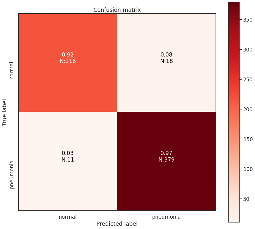
Minimizing both false positives (aka Type-I errors) and false negatives (aka Type-II errors) is important. However, in this situation, it is more damaging in context not to prioritize minimizing false negatives, due to the difference in cost between false positives and false negatives. False positives mean that the healthy child is potentially given extra attention and resources are mis-directed towards them. False negatives mean that a child goes potentially untreated for pneumonia which would be deadly. False negatives are the more important case in this situation to minimize, and it seems this model setup managed to do so. Best case would be ZERO false negatives of course.
My model here appears to mildly outperform the originally cited transfer learning model from the Cell journal article. My transfer-learning model achieves a median accuracy of 94.2% (+1.4), a median sensitivity of 96.2% (+3.0), and a median specificity of 91.0% (+0.9) with the performance difference compared to the Cell model in parentheses. In addition to these estimates the Bayesian dense layers used in this transfer learning setup can also be used to generate confidence intervals on these metrics to better illustrate the performance of the model beyond a singular value. The 95% confidence intervals for accuracy, sensitivity, and specificity are [ 93.6 (+0.8), 94.9 (+2.1) ], [ 95.3 (+2.1), 96.7 (+3.5) ], and [ 90.1 (0.0), 92.7 (+1.7) ], respectively. The values in parentheses are the differences between the same performance metrics from the Cell article model. I also summarize these findings in the table at the bottom of this project article.
I also generate the Receiver Operator Characteristic (ROC) curve for this model. The ROC curve is a useful tool to assess the performance of a diagnostic tools. Theoretically, the best diagnostic tool will have a curve drawn all the way to the top-left, indicating that it has a high true positive rate, and a zero false positive rate at all decision thresholds. With the ROC curve it is possible to compute the Area Under Curve (AUC) value, which statistically describes how well the diagnostic model can perform classifications. The AUC has a minimum and maximum value of 0.0 and 1.0, respectively, with 1.0 indicating a ‘perfect classifier’ that has no false positives or false negatives. A random guess classifier (such as flipping a coin) will have an AUC of 0.5, which is a diagonal line from the bottom left to the top right of the plotted ROC curve. An AUC value less than 0.5 and approaching 0.0 indicates a classifier that performs worse than random-guessing at classification.
I have plotted the ROC curve for my model setup in the figure below, with shaded regions indicating the 95% confidence interval for the ROC curve. This confidence interval was created by resampling the classification probabilities of the test dataset made possible by the Bayesian layers in model. I have also added the median AUC value from these resamples, with the average change in the 95% confidence interval of AUC values. The model i’ve built here has an AUC value slightly lower than the authors of the Cell article model. The authors there achieve an AUC value of 0.968 in their ROC for detecting Pneumonia from Normal chest x-rays. My model’s AUC has a median value of 0.936 (-0.032), with the difference between my model’s AUC and the author’s model AUC in parentheses. This discrepancy in AUC values might be due to my use of class weights in training the model. The author’s in the Cell article do not state that they use class weights in training their model for the pneumonia detection phase.
Benefits of Using Bayesian Models
Ultimately a Bayesian model that is used for single predictions is wasted, as the power of Bayesian models is their capability to model weights and biases as distributions. These distributions can model the uncertainty that exists within the model, and the data itself. It is then possible to assess the capacity of a Bayesian model to perform classifications beyond single prediction instances. In the context of diagnosing Pneumonia in chest x-rays, this means that the output classifications can have probability distributions, which can better inform as to the quality of a final classification. To illustrate this I plot 4 different chest x-rays below, each representing a different type of classification, in the same orientation as a confusion matrix, that is:
| True Negative | False Positive |
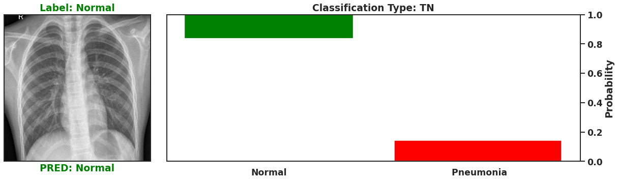 | 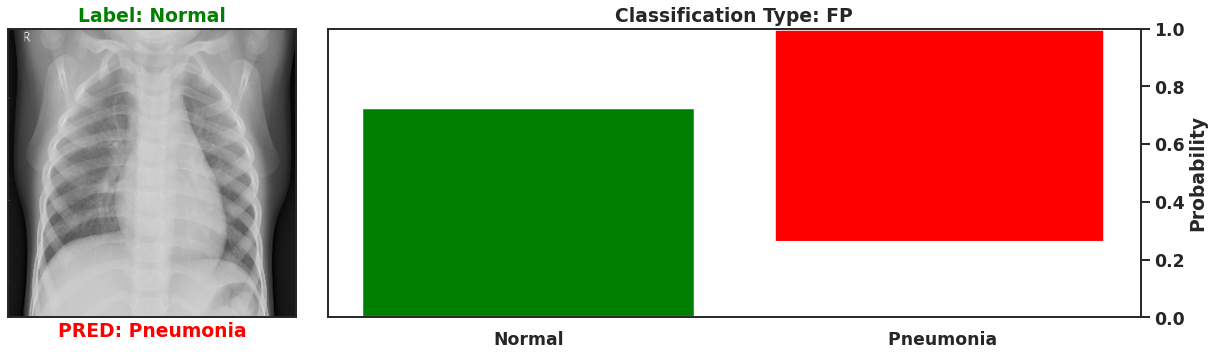 |
| False Negative | True Positive |
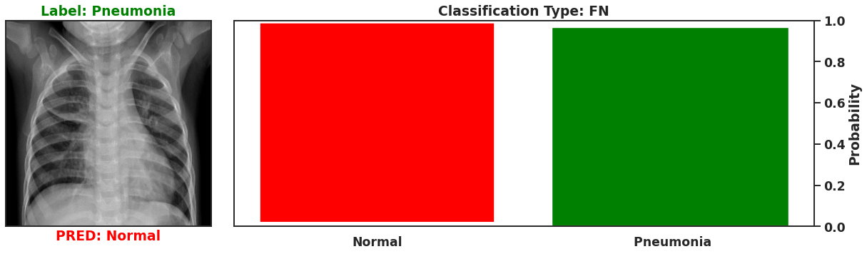 | 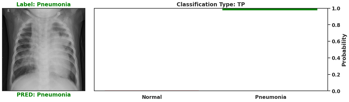 |
These images show that Bayesian neural networks can assess the uncertainty of the classifications it produces, and relay that information as a ‘spread’ in the probabilities of each image being a specific class. Ideally, we’d want the network to be very sure when it classifies negative and positive classes correctly, which means very small spread in those probabilities. This is shown in the true positive Pneumonia detection (bottom right above), and the true negative diagnosis of no Pneumonia (top left above). Counter to being very certain of it’s correct classifications, we want the network to display much larger uncertainty in its incorrect classifications, in the form of a large spread in the class probabilities of each image. This is apparent in the false positive (top right above) and the false negative (bottom left above). This extra information makes the classifications from this neural network more interpretable than just being ‘Pneumonia’ or ‘Normal’ now they have a ‘quality’ as to how reliable the classification can be considered.
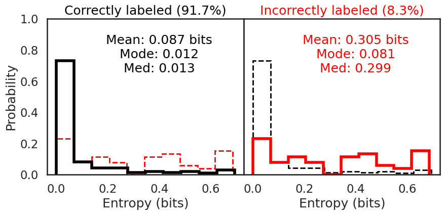
We can also use the classification probabilities to assess the overall performance of the network by calculating the entropy in the classifications. Entropy, as a reminder, is the amount of information that is recoverable from a system. In this sense information is taken to be the amount of heterogeneity. A ‘perfect’ classification of ‘Pneumonia’ would have an entropy of 0.0 as the entirety of all classification probabilities are homogenous and indicating ‘Pneumonia’
I first plot the entropy distributions split on whether the image was correctly or incorrectly classified. The left plot is the entropy distribution of the correctly classified images. The right plot is the entropy distribution of the incorrectly classified images. Each entropy distribution is also plotted in dashed lines to better compare them to each other. The mean, median, and mode for the correctly classified images were 0.087 bits, 0.013 bits, and 0.012 bits, respectively. The mean, median, and mode for the incorrectly classified images were 0.305 bits, 0.299 bits, and 0.081 bits, respectively. The smaller entropy in the correctly classified images illustrates how much more confident the model is in its predictions, since there is little variation in the predictions for each correctly classified image. The incorrectly classified images have an entropy 3.5x to 20x the amount of the correctly classified images. The network isn’t as sure, which means the predictions have more variation, increasing the entropy.
 |
Thanks for reading this far. I enjoyed learning how to make use of pre-trained networks to perform feature extraction as well as managing memory to be able to leverage more out of a smaller personal computer. This project is now accessible as well in a streamlit web app where you can play with adding different types of image noise and manipulating test images in browser with the trained model used here. Hope you enjoyed reading!
Final Summary of Model Performance
| Metric | Cell Article Model | This Project | 95% Confidence Interval |
|---|---|---|---|
| Accuracy | 92.8% | 94.2% ( +1.4) | 93.6% (+0.8), 94.9% (+2.1) |
| Sensitivity | 93.2% | 96.2% ( +3.0) | 95.3% (+2.1), 96.7% (+3.5) |
| Specificity | 90.1% | 91.0% ( +0.9) | 90.1 (0.0), 92.7 (+1.7) |
| AUC | 0.968 | 0.936 (-0.032) | 0.925 (-0.043), 0.946 (-0.022) |